
An elongated cloud of points can look unremarkable from the wrong angle. We see two columns, two axes and some observations. Rotate the paper and something simpler appears: almost all the variation follows one direction.
That image feels like a more useful introduction to PCA than beginning with a covariance matrix. The matrix will come, because it matters. First, though, we should see the problem: finding coordinates that compactly describe how the data varies.
We are not choosing a winning column. A component combines columns. We are not initially looking for the variable that explains a business decision either. PCA does not consult a target when choosing its directions.
Rotate the paper
Imagine two sensors measuring almost the same phenomenon. Their readings rise and fall together, with some noise. Instead of keeping two similar descriptions, we can look for a direction capturing their shared variation and another capturing the remaining differences.
The first principal component is the direction of maximum variance in centered data. The second is perpendicular to it and captures the largest possible variance among the remaining directions. More variables follow the same logic.
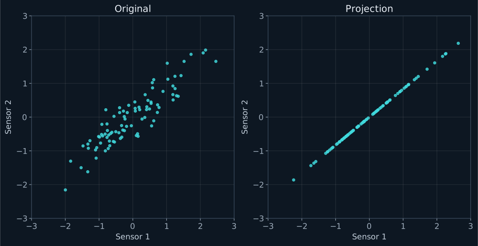
Keeping every component simply changes coordinates. Keeping one gives each observation a single coordinate along that direction. Reconstructing it puts it back on a line. The distance between the original point and its reconstruction shows what we lost.
A projection is not a neutral photograph. Observations that differed along a discarded direction can end up close together. A two-component plot can reveal one structure and hide another. We do not need to distrust every plot; we need to remember what it cannot show.
The size of an axis tells a story too
Change one sensor’s unit from meters to millimeters. The phenomenon stays the same, but its numerical variance grows considerably. PCA on those values can point its first component toward a variable made large by its units.
Centering subtracts the mean. Standardization also divides by the standard deviation. These are different operations. Scikit-learn’s PCA implementation centers features but does not automatically scale them.
Standardization is often helpful when we want different units to participate on comparable terms. It is not a universal obligation. If variables share a unit and their different variability is meaningful, equalizing that variability can remove part of the meaning we hoped to retain.
The choice should not disappear inside a helper function. It is an analytical decision. Changing preprocessing changes the geometry PCA treats as important. Constant variables, unreliable measurements and outliers also deserve inspection before we interpret components.
A percentage that cannot answer every question
Explained variance measures the fraction of total variation captured by each component under the chosen preprocessing. If two components accumulate 95%, we have retained much of that variation. We have not established that we retained 95% of predictive usefulness, causal information or the meaning of the problem.
A low-variance signal could distinguish a rare defect. A high-variance pattern could simply reflect ambient temperature. PCA optimizes its own criterion rather than a universal definition of importance.
To interpret a component, I would examine its coefficients, often called loadings, and revisit the original variables. A name such as “activity level” can be useful if the combination supports it, but the algorithm does not generate that meaning automatically. A direction’s sign can also flip: multiplying a component by minus one does not change the space it describes.
Two components can give us a map. To choose how many to retain, I would inspect cumulative variance, reconstruction residuals and the intended use. For prediction, I would compare no reduction with different alternatives, fitting both scaling and PCA on training data alone.
That comparison should use the same evaluation protocol. A cleaner-looking plot is not evidence that a classifier will improve. Nor should we choose a component count by repeatedly inspecting final test scores. A representation can be useful for explanation and unnecessary for prediction, or the other way around.
A matrix summarizing relationships
Covariance describes how centered columns vary together. Its eigenvectors give PCA directions, and its eigenvalues give variance along those directions. The new coordinates are uncorrelated; that does not generally imply statistical independence.
You do not need to calculate every element manually to use PCA. Understanding the relationship helps explain why the method responds to linear patterns, why scale matters and why dimensionality reduction changes what we can observe.
In the multivariate analysis application you can change variables and inspect the resulting representation. That comparison teaches more than memorizing a single attractive diagram.
The second part connects this geometry to SVD. We will move from a cloud of points to an image and see what reconstructing something with fewer pieces means, without pretending mathematical compression is the same as saving a smaller JPEG.

Found this useful? If you would like to support this space, you can buy me a coffee.
Buy me a coffee Optional support through PayPal. You choose the amount.