
Open a database and you see tables: rows, columns and a few identifiers. At first glance, it looks rather like a spreadsheet. So why call it a relational model instead of simply a collection of tables?
The difference lies in what those tables mean and the rules surrounding them. Storing a value is not enough. We need to know what it represents, which values it can take, how to distinguish one record from another and which connections are valid.
I find a small example more useful than memorizing definitions. We will build a fictional shop. No SQL knowledge is needed to follow along: before writing a query, we want to understand what we are querying. The attribute names stay in Spanish so both language versions share the same data.
A relation is not a link between two tables
Here is our customer information:
| cliente_id | nombre | ciudad | |
|---|---|---|---|
| 1 | Ana | ana@example.com | Sevilla |
| 2 | Bruno | bruno@example.com | Bilbao |
| 3 | Carla | carla@example.com | Sevilla |
| 4 | Diego | diego@example.com | Valencia |
In the relational model, CLIENTES is a relation. We can display it as a table, but the term does not mean the link we will later establish with orders. In everyday language, a relation often means a connection. Here it names the structure holding the data.
Each row is a tuple. The first expresses a fact: customer 1 is called Ana and has that email and city. Each column corresponds to an attribute. The attribute nombre tells us what role the value “Ana” plays in that fact. Without attribute names, we would see values without knowing how to interpret them.
We can write the tuple as ⟨1, Ana, ana@example.com, Sevilla⟩, provided we have specified which attribute each position represents. This is a compact notation, not a requirement to physically store values in that order.
A domain tells us which values make sense
An attribute should not accept just anything. Its domain is the set of atomic values it can take. In this model, atomic means treating a value as a unit rather than a collection of other values that the database must traverse.
For cliente_id, we could define a domain of positive integers. For nombre, nonempty text. For email, text satisfying whatever email requirements we agree on. The values available in a programming data type are not necessarily the values our application should accept.
Orders make this clearer. Suppose estado can only be pendiente, pagado or cancelado: pending, paid or cancelled. Its domain contains those three values. “Blue” is perfectly valid text, but not a valid order status for this shop.
There are predefined domains, such as integers, text and dates, and more specific user-defined domains. A type like INTEGER sets an initial boundary; a condition such as “greater than zero” narrows it.
Domain and attribute are not synonyms either. telefono_personal and telefono_trabajo might share a phone-number domain while expressing different things. The domain tells us which values are allowed; the attribute tells us what they mean here.
This also explains why putting "600111222, 600333444" into one cell is a poor way to represent two phone numbers we need to query separately. We have turned a collection into text that must later be interpreted. If each phone needs its own identity in our queries, another relation can hold one tuple per customer and phone. A string does not stop being atomic merely because it contains commas; the problem is hiding several independently meaningful facts inside it.
Schema and extension: the shape and the contents
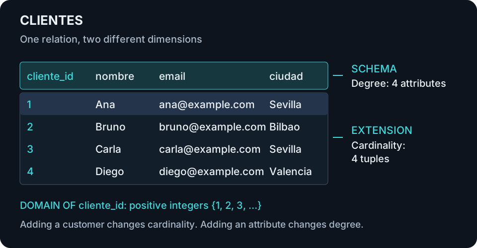
A relation schema, also called its intension, describes its structure. We usually write the relation name followed by its attributes:
CLIENTES(cliente_id, nombre, email, ciudad)A full definition also associates domains and specifies keys and constraints. The extension is the set of tuples present at a particular moment: here, the four rows in the table.
If Elena registers tomorrow, the extension changes. If we add an attribute called fecha_alta, the registration date, the schema changes. Adding another customer is different from deciding to record a new kind of information.
A relation can be empty and still have a schema. A new shop might have no customers yet, but we already know what information its first customer record will contain.
The schema of one relation is not the schema of the whole database. The latter collects relation definitions and the constraints connecting them. Some database systems also use schema for a namespace containing tables and other objects. The context matters.
Degree and cardinality: columns are not rows
The degree of a relation is the number of attributes in its schema. CLIENTES has degree 4. Its cardinality is the number of tuples in its extension: currently also 4, but that is a coincidence.
Add a hundred customers and the degree stays at 4 while cardinality becomes 104. Add fecha_alta without registering anyone else and the degree becomes 5 while cardinality remains 4.
You may also encounter cardinality when discussing one-to-many associations. There it describes participation in an association; here it counts tuples in a specific relation. These are different uses of the same word.
What a relation does not promise
The extension is a set, so the relational model has no duplicate tuples. Individual columns can repeat: both Ana and Carla live in Sevilla. What cannot repeat is the complete tuple.
There is no inherent “first tuple” either. Rearranging rows on screen does not change the relation. If we want customers displayed alphabetically, we must request that ordering. Attributes are identified by name and have no compulsory logical order, although a written table or tuple needs a layout for us to read.
SQL practice and relational theory are not identical. An SQL table without constraints can accept duplicate rows, and queries can return duplicates even when their source tables have keys. DISTINCT removes duplicates from a result; ORDER BY specifies its presentation order. The PostgreSQL documentation on select lists explains the former. Looking like a table does not automatically make an SQL object satisfy every theoretical property of a relation.
Identifying is different from describing
All four customers currently have different names. Could nombre be a key? Not if the shop allows another Ana to register tomorrow. A key must work across the valid states of the database, not merely the sample currently on screen.
A superkey is a set of attributes that uniquely identifies each tuple. If cliente_id is unique, both {cliente_id} and {cliente_id, nombre} are superkeys. The second works, but includes an attribute we do not need.
A candidate key is a minimal superkey: removing any of its attributes destroys that identifying property. Minimal does not mean the shortest among all keys; it means no attribute within that key is redundant.
Suppose the shop also requires a unique, mandatory email per customer. Then {cliente_id} and {email} are candidate keys. We choose {cliente_id} as the primary key, leaving {email} as an alternate key. If shared emails were allowed, email would no longer qualify as a candidate key. This depends on the system’s rules.
Keys can be composite. In LINEAS_PEDIDO, order lines, {pedido_id, numero_linea} could identify each line. Orders 101 and 102 can both have a line numbered 1, but one order cannot have two line-1 records. Neither attribute suffices alone; together they do.
We still need to prevent an order from naming a nonexistent customer or carrying an amount our shop does not accept. That concerns valid database states rather than table layout. It is the subject of part two.

Found this useful? If you would like to support this space, you can buy me a coffee.
Buy me a coffee Optional support through PayPal. You choose the amount.