
At eight in the morning there are sixty bicycles at station A, thirty at B and ten at C. Someone needs to know how many will be available after the next period. Not where each bicycle will end up, but how the fleet will be distributed.
We could track every vehicle and simulate its journeys. We can also begin with something smaller: the probabilities of moving between stations. A Markov chain turns that description into a model we can follow, calculate and discuss.
Everything below is hypothetical. The probabilities do not come from a real service, and a period is an abstract unit rather than an hour calibrated from data. I prefer stating this before an attractive chart gives the model more authority than it deserves.
Three states and a reading convention
Suppose a bicycle at A has a 60% chance of remaining there, a 30% chance of moving to B and a 10% chance of reaching C. From B the probabilities are 20%, 50% and 30%; from C they are 40%, 20% and 40%.
| Origin → destination | A | B | C |
|---|---|---|---|
| A | 0.60 | 0.30 | 0.10 |
| B | 0.20 | 0.50 | 0.30 |
| C | 0.40 | 0.20 | 0.40 |
Each row sums to one. A bicycle must reach one of the states we have defined. If vehicles can leave the system or break down and we omit those states, the matrix does not describe the complete situation.
I will use row vectors, so evolution is x(t+1) = x(t) P. Column vectors and a transposed matrix work too. Neither convention is cleverer, but mixing them gives incorrect results. Always accompany the matrix with a sentence: rows are origins, columns are destinations.
The Markov assumption says that, given the current state, the distribution of the next one does not require the entire previous history. It does not say the past never matters in reality. We are trying to summarize the relevant information in our chosen state.
If a recently repaired bicycle behaves differently from one that has gone months without maintenance, “being at A” may not contain enough information. The model does not automatically discover this. We must detect the pattern and expand the state description or choose a different approach.
Calculate the first move by hand
Of the sixty bicycles initially at A, we expect 36 to stay there, 18 to reach B and 6 to reach C. The thirty at B contribute 6, 15 and 9. The ten at C contribute 4, 2 and 4. Adding these gives 46 at A, 35 at B and 19 at C.
This is an expected distribution. One particular realization might be 44, 38 and 18; that illustrative alternative is not an executed simulation. An expectation does not oblige individual vehicles to obey a table.
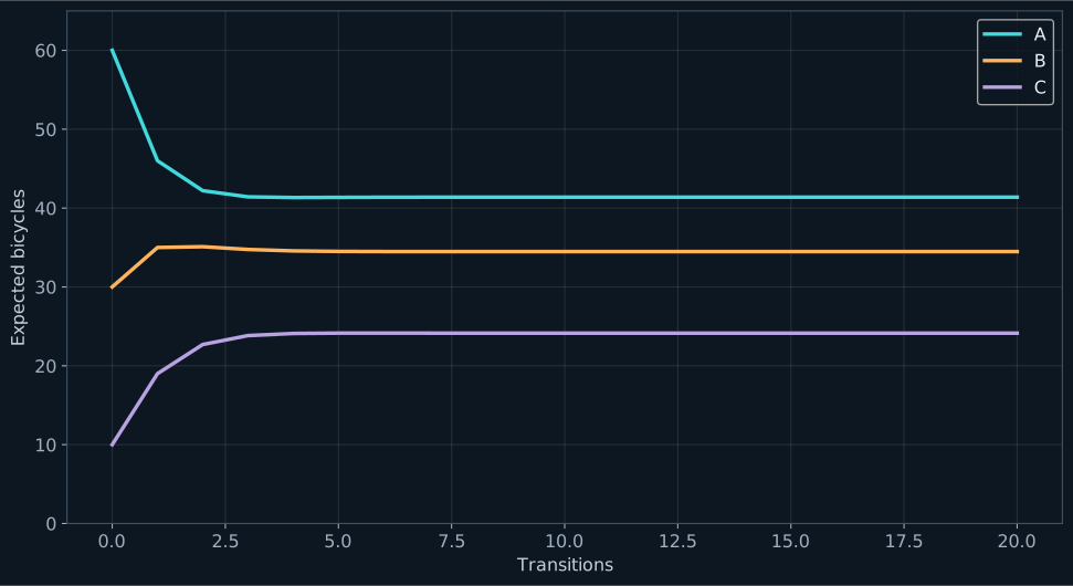
This distinction gives us two questions. One asks where the fleet concentrates on average. Another asks how likely a station is to run out of bicycles. The second requires variability, not just an expected-value curve. A station averaging ten bicycles can still face a meaningful shortage risk, depending on the journeys.
The first step needs just one multiplication:
import numpy as np

P = np.array([[.6, .3, .1], [.2, .5, .3], [.4, .2, .4]])
x = np.array([60., 30., 10.])
assert np.allclose(P.sum(axis=1), 1)
print(x @ P)  # [46. 35. 19.]
There is no training, hyperparameter search or hidden neural network. The model sits in the probabilities we put on the table. That transparency is useful: we can ask where each probability came from and what happens if it stops being reasonable.
Repetition is not a forecast guarantee
To advance several periods, we multiply by the same matrix again. This assumes constant transition probabilities: a homogeneous chain. If morning journeys mostly head toward B and evening journeys mostly return, a single matrix could hide precisely the behavior we care about.
We have not modeled docking capacity, shared routes or redistribution interventions. Each bicycle evolves without station occupancy changing its probabilities. A full station breaks that convenience: repeatedly multiplying a matrix cannot force reality to fit.
There is a useful middle ground between rejecting such a simple model and treating it as a complete service simulator. We can use it to expose assumptions, compare hypothetical changes and identify which observations we would need before moving further. A probability table estimated over a whole year would need particular scrutiny if the decision concerns tomorrow morning.
In my mobility simulator you can explore expected evolution alongside random journeys. The comparison is a good way to test intuition before turning a calculation into a recommendation.
One uncomfortable question remains. Even if the distribution stabilizes, does it leave us with a useful fleet? In the next part we will introduce a breakdown state. The equilibrium can remain mathematically impeccable while becoming operationally disastrous.

Found this useful? If you would like to support this space, you can buy me a coffee.
Buy me a coffee Optional support through PayPal. You choose the amount.