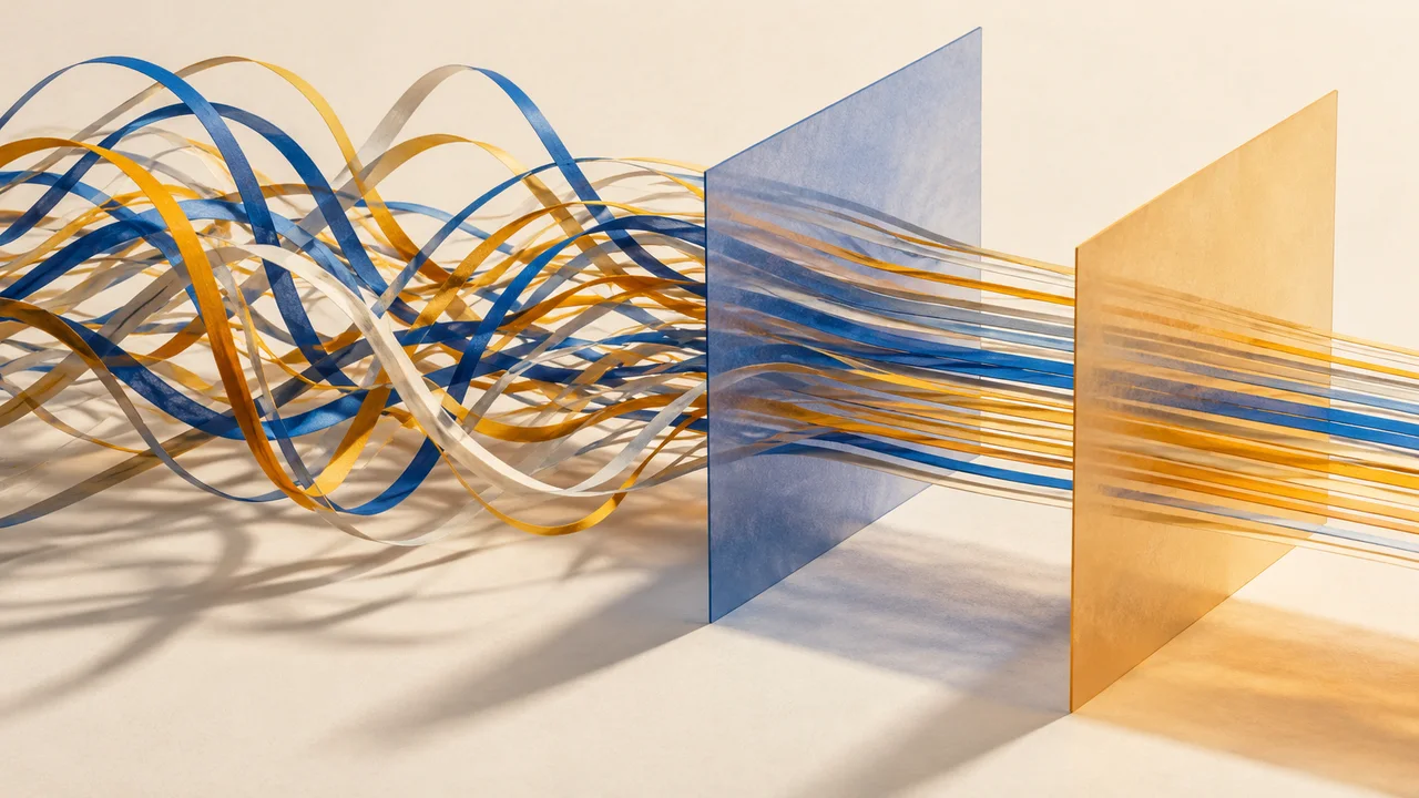
Look closely at a grayscale image. Behind the drawing is a table of intensities: a row and a column for every pixel position. Turning a picture into a matrix does not make it less interesting. It lets us ask a different kind of question.
For instance, can we approximately reconstruct it using fewer numbers? Not by dropping random pixels, but by finding patterns that describe many pixels at once.
An image as a sum of layers
Singular value decomposition writes a matrix as A = U Σ Vᵀ. The columns of U and V provide directions; the diagonal of Σ contains nonnegative singular values ordered from largest to smallest.
We can also read this as a sum of pieces. Each is a column vector multiplied by a row vector and weighted by its singular value. Each has rank one. Add all the required pieces and they reconstruct the matrix. Keep the first k and we obtain an approximation of rank at most k.
This reading is less intimidating than three letters together. Early layers capture strong patterns. Later ones can add contours, textures or subtle differences. They are not semantic objects: SVD does not automatically separate “the house,” “the tree” and “the sky.”
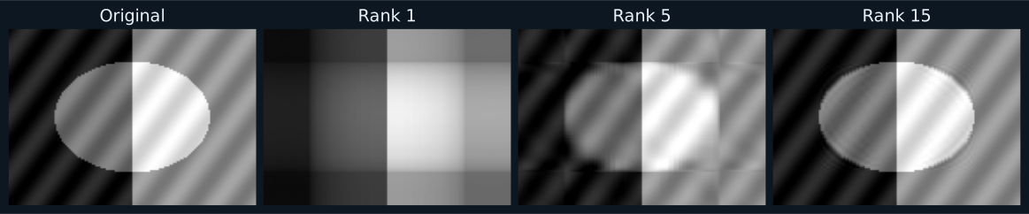
Increasing k usually makes the image look closer to the original, but “closer” needs a criterion. Truncated SVD provides an optimal rank-limited approximation in matrix norms such as the Frobenius norm. That measures numerical differences, not the importance of a detail to a person.
A tiny piece of text may be essential for reading a sign while contributing little to the image’s total energy. The method does not know that losing the text changes the meaning. This is the first part’s warning in another form: preserving most variation does not preserve all useful information.
Try it without someone else’s photograph
We can experiment without downloading pictures or reusing textbook figures. Construct a small matrix with a geometric shape and some texture:
import numpy as np

y, x = np.mgrid[-1:1:100j, -1:1:140j]
A = .2 + .4 * (x > 0) + .3 * (x*x + y*y < .4)
A = A + .08 * np.sin(17*x + 9*y)
U, s, Vt = np.linalg.svd(A, full_matrices=False)
k = 5
approx = (U[:, :k] * s[:k]) @ Vt[:k]
print(np.linalg.norm(A - approx, "fro"))
This produces a matrix approximation, not a compressed file ready for distribution. To visualize it fairly, use the same intensity scale for the original and every reconstruction. If each panel adjusts its contrast independently, the plot can make a poor reconstruction look better than it is.
Our matrix contains 14,000 entries. Storing truncated factors requires k × (100 + 140 + 1) numbers: 1,205 with five components. This compares numerical entries at equal precision. It does not promise a particular reduction in bytes against PNG or JPEG, which already use other techniques and structures.
If we reconstruct the entire matrix and save it in a format that does not retain the factors, we are storing all its pixels again. Using fewer components to calculate an image does not guarantee a smaller resulting file.
The connection to PCA
For a centered observation matrix X, principal directions can be obtained from the right singular vectors. Squared singular values divided by n − 1 give component variances. Projected coordinates are U Σ.
PCA and SVD are not exact synonyms. SVD factorizes any matrix; PCA is a statistical procedure on centered data, with preprocessing and interpretation decisions. Directly approximating an image is not necessarily performing PCA on observations.
The connection allows PCA to be calculated without explicitly forming the covariance matrix. It is numerically useful and keeps the two techniques from looking like unrelated recipes. NumPy’s SVD documentation describes the factors and dimensions returned by the function used here.
Look at the residual too
Instead of inspecting only the reconstruction, look at A − approx. What disappeared: noise, edges, a small structure? With tabular data, we can also examine errors by observation and feature. A low mean can hide a poorly represented group.
Different downstream tasks give that loss different significance. A visualization may tolerate approximate coordinates that would be unsuitable for identifying a rare event. A compression exercise can reveal geometry without making a claim about predictive accuracy. Naming the task prevents one success from standing in for another.
Dimensionality reduction is not always necessary. A larger original representation may be easier to explain and cheap enough to use. Many columns alone do not justify PCA; redundancy, noise, sample size and purpose all matter.
I would keep the habit of looking at both sides of an approximation. The reconstruction tells us what survived. The residual tells us the price of simplifying. Without that second picture, a compact representation can too easily pass for a complete explanation.

Found this useful? If you would like to support this space, you can buy me a coffee.
Buy me a coffee Optional support through PayPal. You choose the amount.