
Return to our hundred bicycles. With only three stations, availability is conserved. We can debate their distribution, but no vehicle disappears. That convenience ends as soon as a bicycle can break down.
We add a fourth state, T: out of service, awaiting repair. It is not a station where someone can collect a bicycle. Counting it as availability would be wrong even though it belongs to the total fleet.
An equilibrium we should not celebrate
Assume a 5% breakdown probability in each transition for every operational bicycle. The remaining 95% moves between stations using the first part’s probabilities. Without repairs, any bicycle entering T stays there. T is an absorbing state.
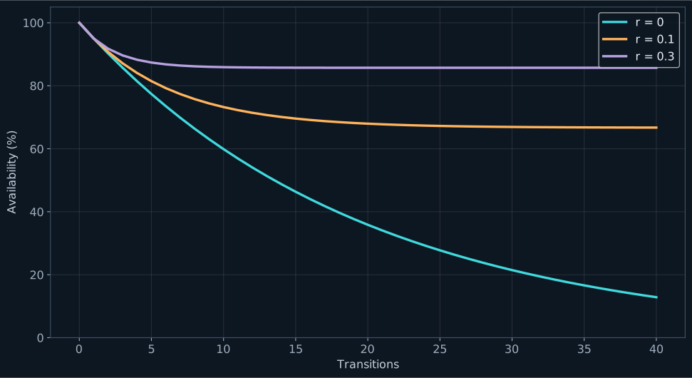
No new vehicles arrive and none are permanently removed. All hundred remain accounted for, but fewer and fewer can be used. Because the breakdown risk is identical across stations, expected availability after t steps is 100 × 0.95^t.
After twenty transitions, approximately 35.85% of the fleet remains operational. This is not a company’s estimate or an observed rate. It is the exact consequence of our hypothesis. Keep the model running indefinitely and availability tends to zero.
The system has a stationary distribution: everything in the workshop. It is mathematically in equilibrium. As a mobility service, it is useless. This is why I would not interpret “stable” as “good” without asking what the states mean.
Repair changes the story
Now a bicycle in T can return to service with probability r per period. To study availability alone we can group A, B and C into an operational state O. This aggregation is valid in our example because all stations have the same breakdown risk. Different risks would not automatically allow it.
| Origin → destination | O | T |
|---|---|---|
| O | 0.95 | 0.05 |
| T | r | 1 − r |
At equilibrium, the expected flow breaking down equals the flow being repaired. If q is the operational fraction, 0.05q = r(1 − q), giving q = r / (r + 0.05).
With r = 0.10, the limit is two thirds of the fleet. With r = 0.30, it is approximately 85.71%. We have not shown that tripling a maintenance budget produces this improvement. r is a transition probability. Connecting it to staffing, shifts or money requires another model and data.
import numpy as np

for repair in [0., .1, .3]:
    P = np.array([[.95, .05], [repair, 1 - repair]])
    x = np.array([1., 0.])
    for _ in range(20):
        x = x @ P
    print(repair, round(x[0] * 100, 2))
This reports expected availability after twenty steps, not necessarily the limit. Confusing the two is easy when a curve looks flat. A repair probability is also not a fixed number of daily repairs. A capacity-limited workshop cannot automatically repair a constant fraction of any queue.
A limit needs conditions
The three-station chain has positive entries. In this finite setting, there is a unique stationary distribution and convergence toward it. A general chain does not have to behave that way.
Consider two stations where every bicycle must move to the other at each step. The distribution can alternate forever. A half-and-half stationary distribution exists, but starting with all bicycles in one station does not converge to it. Solving πP = π does not prove that every evolving distribution reaches that solution.
Not every part of a system needs to communicate either. Two isolated groups of states can make the long-term distribution depend on the starting point. Before announcing a final forecast, inspect reachability, closed classes and periodicity. These properties are discussed in the Markov-chain chapter of Grinstead and Snell’s open probability textbook.
Toward a maintenance decision
The useful next step is not another decimal place. It is asking whether the states represent the service we need to manage. Do breakdowns require equal work? Can the workshop handle the queue? Does demand change on weekends? Does redistribution have a cost?
I would separate availability from location. Eighty operational bicycles are not necessarily where users need them. I would then compare scenarios over a specified horizon: a decision for tomorrow cannot be justified by a distant equilibrium alone.
Even a small model can help decide what to measure next. If changing r matters far more than changing route probabilities, maintenance data deserves attention. If station shortages dominate while total availability remains high, redistribution deserves another model. Neither conclusion follows just from admiring the smoothness of a curve.
This is what interests me about these models. They do not promise to describe the whole world, but they turn assumptions into visible consequences. Sometimes the most useful consequence is discovering that the equilibrium we were seeking was actually the problem.

Found this useful? If you would like to support this space, you can buy me a coffee.
Buy me a coffee Optional support through PayPal. You choose the amount.