
In 1951, Andrew Huxley had to solve the equations of a squid nerve cell by hand. The computer he had hoped to use had broken down, and the calculation, performed with a hand-cranked mechanical machine, took more than three weeks. Together with Alan Hodgkin, he was developing a mathematical model to explain how neurons generate and transmit electrical impulses.
From a neuron model to the work of an AI
Hodgkin and Huxley wanted to explain how a neuron produces an electrical impulse. They represented its membrane as an electrical circuit and wrote equations describing how it worked. They then calculated the activity predicted by those equations and compared it with measurements from the cell.
One part of the model described potassium channels opening: small passages in the membrane through which ions flow, contributing to the electrical current. The researchers found that reproducing the measurements required a variable in their equations to appear raised to the fourth power, meaning four copies of the variable multiplied together. Other powers gave less accurate results.
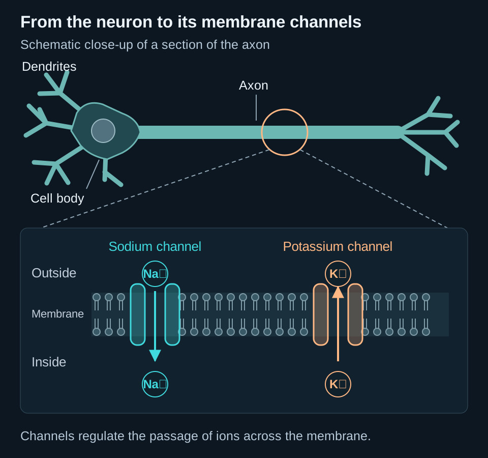
At that point, they knew the mathematical result but could not observe the channel’s structure. They sought a physical explanation: perhaps opening required several particles to move into position. Decades later, research into a potassium channel revealed four parts surrounding a central passage. This finding was consistent with their hypothesis, although the equation alone did not establish that the channel had that structure.
The connection to AI lies in this process of proposing equations and testing them. An AI system could receive the neuron’s measurements and a description of the problem, propose candidate equations and use a program to simulate the activity each predicts. It could then fit their parameters, compare simulations with measurements and revise equations that perform poorly. Here, AI would be the tool helping to build and evaluate the scientific model of the cell.
Interpreting a fourth power proposed by AI would require knowing which other relationships it tested and how they compared with measurements. That comparison gave Hodgkin and Huxley a reason to investigate the meaning of their equation. If several alternatives performed equally well, the data would not yet justify choosing a single explanation of the channel.
Building, fitting and interpreting
The neuron example helps distinguish three tasks. First we choose equations; then we find values for their parameters; finally we investigate what they let us say about the cell.
| Phase | What we do | In the neuron model |
|---|---|---|
| Building | Choose variables and their relationships | Decide how to represent channels opening |
| Fitting and inference | Find values compatible with measurements | Estimate how much each channel type contributes to the current |
| Interpretation | Investigate what the results mean | Test whether a mathematical relationship reflects a channel mechanism |
We will use M for the model structure: the equations we have chosen. θ denotes its parameters, the quantities whose values we need to estimate. D denotes observed data, such as measurements of the neuron’s electrical activity.
Changing a conductance—a measure of how easily current flows—changes a parameter θ. Replacing the fourth power with another relationship changes the structure M. This distinction matters when discussing uncertainty: we may be unsure about values within an equation or about the equation itself.
Many parameter settings can explain one observation
Imagine dinner for four people. We know the menu and the price of each dish, but all we have left is the total bill: €120. Can we work out what each diner ordered?
Several orders are possible. All four diners might have chosen a €30 dish. Or one might have ordered a €60 dish and the other three a €20 dish each. Both combinations add up to €120. The total rules out some orders, but does not identify a single one.

A neuronal model presents a similar problem. We measure the cell’s electrical activity, just as we know the total bill. We want to infer the parameter values that produced that activity, just as we try to reconstruct each person’s order. Different parameter combinations can produce almost identical signals, just as different orders can add up to the same bill.
Bayesian inference lets us assess these alternatives by combining observations with prior information. Returning to dinner, suppose we know the diners usually choose mid-priced dishes and rarely order the most expensive option. We would not necessarily assign equal probabilities to all orders totalling €120. The total tells us which orders fit; prior knowledge also affects which we consider more likely. Those preferences provide information beyond the total bill.
Bayes’ rule expresses this update. For a fixed model structure M:
p(θ | D, M) ∝ p(D | θ, M) · p(θ | M)
Posterior ∝ likelihood × prior
In this example, D is the €120 bill; θ represents each diner’s order; and M contains our fixed rules: four diners, one dish each and the menu prices.
- Prior, p(θ | M): the probability assigned to each order before seeing the total, based on what we know about the diners.
- Likelihood, p(D | θ, M): the probability of a €120 bill if that were the order. In this example without errors or extra charges, an order totalling €80 is ruled out, while one totalling €120 is compatible.
- Posterior, p(θ | D, M): the updated probabilities of the orders after incorporating the observed bill. Several alternatives may remain.
The symbol ∝ means “is proportional to”: we multiply the likelihood by the prior, then normalise the result to obtain a probability distribution. The bar | means “given”: p(θ | D, M) refers to the parameters given the observations and a fixed model.
The difference between likelihood and posterior becomes clearer when we change the question. “If they ordered these dishes, what bill would we expect?” goes from order to total. “Given the total, what might they have ordered?” goes in the inverse direction. In a scientific model, Bayes helps us move from measurements to a distribution of possible parameters without assuming there is only one answer.
In a neuronal model, increasing one parameter and decreasing another may leave the signal almost unchanged. The posterior represents that uncertainty. Calculating it usually involves approximations, such as methods that sample the distribution without visiting every possible value.
Simulation-based inference: learning the inverse direction
At dinner, going from order to total is straightforward: add the prices. For the neuron, we can also enter parameters into a program and calculate the electrical signal they would produce. That program is a simulator of the scientific model.
The difficulty arises when evaluating the likelihood. A complex simulator may generate signals with random variations without offering a practical way to evaluate the probability of real measurements. Generating a possible signal and calculating the probability of an observation are different operations.
Simulation-based inference, or SBI, helps address these cases. One approach, neural posterior estimation, uses a network trained on examples from the simulator.
Training and using the network
- Choose many parameter combinations. For the neuron, these might be different sodium and potassium conductances within the ranges we want to investigate.
- Simulate the activity for each combination. Retain the parameters and the electrical signal each simulation produces.
- Train a network on these pairs. It learns to associate signals with a distribution of parameters that could have generated them.
- Supply a real measurement. The network returns an approximation to the distribution of parameters compatible with that observation, under the model and prior used.
The simulator generates signals from parameters; the network helps infer parameters from signals. The network learns from the simulator’s examples, which represent our model of the cell.
qφ(θ | D) ≈ p(θ | D, M)
The network approximates the posterior
We keep D for data: simulated signals during training or real measurements when using the network. θ denotes the scientific parameters and φ the network’s weights. The symbol ≈ indicates an approximation; model M remains fixed.
Generating simulations and training the network can be costly. Afterwards, we can reuse it to analyse new measurements within its learned domain. This is amortised inference: much of the cost occurs initially. A signal very different from the simulated examples may require more examples or revisions to the model.
Checking the results
We can use simulated signals with known parameters to assess whether the network reports appropriate uncertainty. This helps check its calibration.
We can also draw parameters from the posterior, generate new signals and compare them with real measurements. These posterior predictive checks reveal whether the model reproduces important features of the observed activity.
SBI includes other approaches that approximate the likelihood or compare probabilities of data under different parameters; not all use neural networks.
The equations are uncertain too
So far we have kept the neuron’s equations fixed and searched for their parameter values. But we could also ask whether channel opening should be represented by a fourth power or another relationship. That means comparing different scientific models.
It helps to distinguish these two levels:
- Parameter uncertainty: we have chosen equations, but several combinations of values reproduce the measurements.
- Structural uncertainty: different equations reproduce the measurements, and we do not know which best represents the system.
AI can help explore the second level. An agent using a language model can write code for several simulators, execute them and compare their results with data. Evaluating each proposal also requires fitting or inferring its parameters. When a proposal fails, the agent can revise its equations and try again.
If two structures explain the same measurements, we need a way to assess their support. Choosing only the best-fitting one can hide other plausible explanations.
The comparison can also be expressed through Bayes’ rule:
p(M | D) ∝ p(D | M) · p(M)
Model posterior ∝ evidence × prior
We now update the probability of M, the model structure. p(M) expresses prior assumptions about the structures considered. p(D | M) is the evidence: it summarises how a model explains the data by considering its parameters according to their prior, rather than assessing only its best fit.
For example, one equation might reproduce measurements only with precisely tuned parameters, while another does so across a broader set of plausible values. Evidence accounts for that difference. Results depend on the chosen priors; counting parameters alone cannot determine which model receives more support.
A collection of equations generated by an agent is not, by itself, a Bayesian distribution. An agent proposing an equation repeatedly does not establish its scientific probability: we need to define how each alternative is evaluated and weighted.
Several models may also agree because they share the same error. If all omit an important cell mechanism, they could make the same incorrect prediction. Agreement needs to be assessed in light of shared assumptions.
An experiment that separates two explanations
To see how disagreement guides a measurement, consider a hypothetical example. We apply a stimulus of intensity x and measure a response y. We have tested only weak stimuli, and within that range the response appears to grow along a straight line.
There are at least two possible explanations:
- Linear model: y = ax + b + ε. Each increase in x produces the same increment in the response. Parameter a specifies how much y grows; b is its value when x is zero.
- Saturating model: y = c(1 − e−kx) + ε, with positive c and k. The response grows initially but approaches a limit c. Parameter k controls how quickly it approaches that limit.
In both equations, ε represents variations treated as noise. For small x, the start of the saturating curve resembles a straight line. Mathematically, for small kx, 1 − e−kx ≈ kx. The two models can therefore give very similar results for the weak stimuli measured so far.
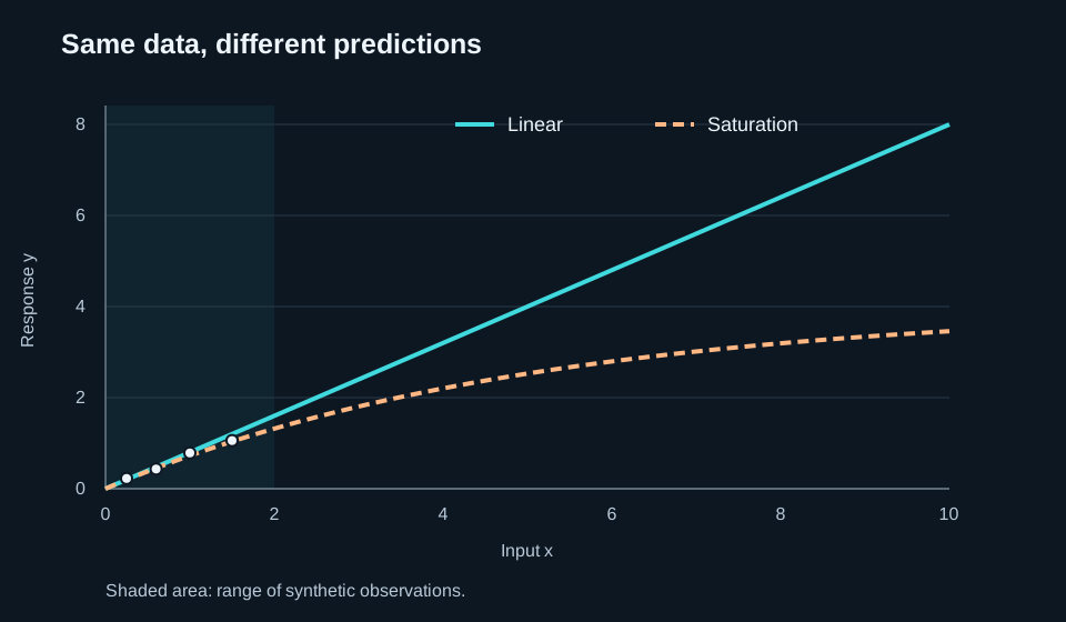
Taking many more measurements with those same stimuli may improve precision without revealing whether the response eventually saturates. A measurement with a stronger stimulus, within valid experimental conditions, would test a specific difference: the linear model predicts continued growth at the same rate, while the other predicts growth slowing down.
AI could identify that range as a useful place to measure. Researchers would decide how to conduct the experiment and compare its outcome with the two predictions.
Distinguishing models and distinguishing parameters
The example compares two structures. Within one structure, parameter values can also be difficult to distinguish. Near the origin, the saturating model behaves approximately as y = ckx: observations inform us about the product ck, but may leave considerable uncertainty about c and k separately.
Identifiability concerns whether observations allow a model’s parameters to be distinguished. Structural identifiability asks this question under ideal conditions; practical identifiability considers real-data limitations such as noise and the number of measurements. If two parameters produce exactly the same observable effect, repeating the same measurement more precisely will not separate them.
Interpreting a model requires testing it
Beyond changing stimulus intensity, we can intervene on a cell mechanism: for example, blocking some of its sodium channels.
First we simulate the block. Two models that reproduced the original activity might predict different changes. Their disagreement indicates which effect would be useful to measure in the cell. We then conduct the experiment and check which models remain compatible with observations.
This begins to evaluate the biological explanation we attach to the equations. Correctly predicting the effect of a channel block supports a model’s representation of that mechanism. One intervention does not confirm every detail, but provides a different test from fitting the original activity.
From one neuron to whole systems
Modelling a brain also requires representing how neurons connect and how their activity affects one another. A connectome maps those connections, but knowing that two neurons connect does not tell us how strongly one affects the other. We still need to represent cells, assign values to connections and compare simulated activity with measurements.
AI can help build and evaluate many models of that system. To investigate a connection, we could simulate removing it in each model and examine predicted behavioural changes. Widely differing answers would mean that the function we assign to the connection depends on unresolved assumptions.
This comparison of alternatives is also used elsewhere: climate simulations examine how projections change with assumptions, while particle physics measurements rule out versions of a theory and leave others open.
What we should ask of scientific AI
AI can propose equations and find parameters that reproduce measurements. For that result to help science, it should also show which other explanations could fit and what observation would distinguish them.
For the neuron, this means explaining which equations were tested, what each predicts and how the signal would change if a channel were altered. Researchers can then choose what to measure and use the result to revisit the explanations.
The value of scientific AI lies not only in finding an answer, but in helping identify the experiment that can test it.
Source
This independently written article draws on the study document “Enseñar a la IA a construir modelos científicos”: Teaching AI to build scientific models, by Jakob Macke, Daniel Gedon and Stefan Wahl, in Anthropic Research.

Found this useful? If you would like to support this space, you can buy me a coffee.
Buy me a coffee Optional support through PayPal. You choose the amount.